Chapter 2 Causal Graphs
2.1 The Fork
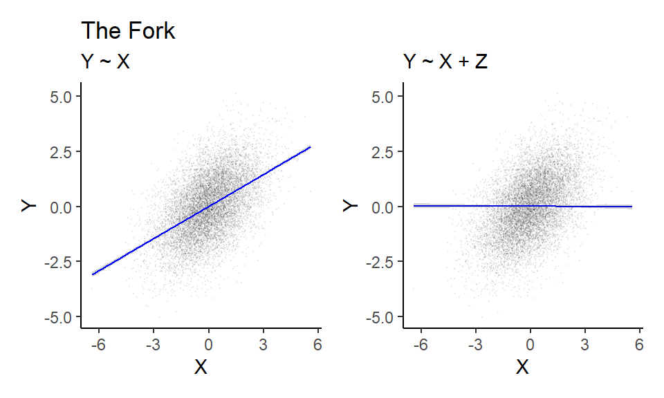
We first simulate some data from the simple ‘Fork’ DAG.
set.seed(1747)
n <- 1e4
bZ <- 1
Z <- rnorm(n, 0, 1)
X <- Z*bZ + rnorm(n, 0, 1)
Y <- Z*bZ + rnorm(n, 0, 1)
We then write a function for fitting and plotting our models that we can re-use for the ‘Pipe’ and ‘Collider’ scenarios. This function depends on the ggplot2 (Wickham et al. 2019) and patchwork (Pedersen 2024) packages.
library(ggplot2)
library(patchwork)

plot_scat <- function(data, title){

# Y ~ X
p1 <- ggplot(data, aes(x=X, y=Y)) +
  geom_point(alpha = 0.05, size = .1) +
  geom_smooth(method='lm', color = "blue", linewidth = 0.5) +
  theme_classic() +
  labs(title = title, subtitle = "Y ~ X")

# Y ~ X + Z
model <- lm(Y ~ X + Z, data = data)
new_data <- transform(data,
                      Z = 0)
predictions <- predict(model, newdata = new_data, interval = "confidence")

p2 <- ggplot(data, aes(x = X, y = Y)) +
  geom_point(alpha = 0.05, size = .1) +
  geom_line(data = new_data, aes(y = predictions[, "fit"]), linewidth = 0.5, color = "blue") +
  geom_ribbon(data = new_data, aes(ymin = predictions[, "lwr"], ymax = predictions[, "upr"]), alpha = 0.2) +
  theme_classic() +
  labs(subtitle = "Y ~ X + Z")

return(p1 + p2)
}
We then apply the function to the simulated data.

2.2 The Pipe
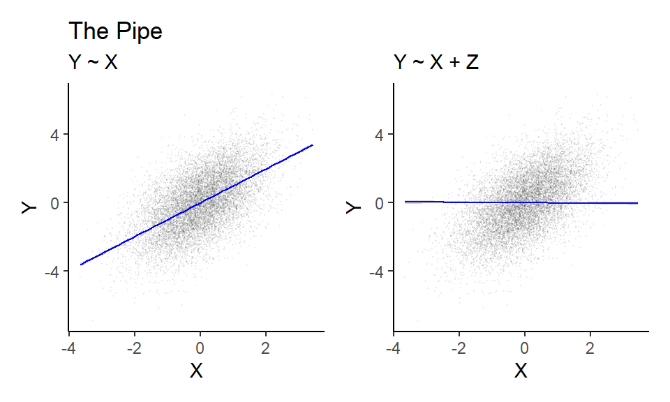
Similarly to above, we simulate data from the ‘Pipe’ DAG…
set.seed(1747)
n <- 1e4
bZ <- 1
bX <- 1
X <- rnorm(n, 0, 1)
Z <- X*bX + rnorm(n, 0, 1)
Y <- Z*bZ + rnorm(n, 0, 1)
… and then apply our custom fitting and plotting function.

2.3 The Collider
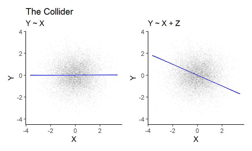
Exactly the same approach as above.
set.seed(1747)
n <- 1e4
bX <- 1
bY <- 1
X <- rnorm(n, 0, 1)
Y <- rnorm(n, 0, 1)
Z <- X*bX + Y*bY + rnorm(n, 0, 1)

plot_scat(data = data.frame(Y=Y, X=X, Z=Z), title = "The Collider")
2.4 Post-treatment bias
Again, following the same approach, we simulate data from the post-treatment DAG.
set.seed(1747)
n <- 1e4
bZ <- 1
bX <- 0.5
bY <- 1
Z <- rnorm(n, 0, 1)
X <- Z*bZ + rnorm(n, 0, 1)
Y <- Z*bZ + X*bX + rnorm(n, 0, 1)
P <- Y*bY + rnorm(n, 0, 1)
Next, we fit two models: One that adjusts for the post-treatment variable P…
##
## Call:  glm(formula = Y ~ X + Z + P, data = data.frame(Y = Y, X = X,
##     Z = Z, P = P))
##
## Coefficients:
## (Intercept)            X            Z            P
##     0.01018      0.25354      0.50133      0.48813
##
## Degrees of Freedom: 9999 Total (i.e. Null);  9996 Residual
## Null Deviance:       34040
## Residual Deviance: 4895  AIC: 21240
… and another that doesn’t.
##
## Call:  glm(formula = Y ~ X + Z, data = data.frame(Y = Y, X = X, Z = Z))
##
## Coefficients:
## (Intercept)            X            Z
##    0.007601     0.495594     0.987202
##
## Degrees of Freedom: 9999 Total (i.e. Null);  9997 Residual
## Null Deviance:       34040
## Residual Deviance: 9793  AIC: 28180
We see that only the latter model picks up the correct estimate for X, which was 0.5 in this case.
2.5 Session info
## R version 4.4.1 (2024-06-14 ucrt)
## Platform: x86_64-w64-mingw32/x64
## Running under: Windows 10 x64 (build 19045)
##
## Matrix products: default
##
##
## locale:
## [1] LC_COLLATE=Danish_Denmark.utf8  LC_CTYPE=Danish_Denmark.utf8
## [3] LC_MONETARY=Danish_Denmark.utf8 LC_NUMERIC=C
## [5] LC_TIME=Danish_Denmark.utf8
##
## time zone: Europe/Copenhagen
## tzcode source: internal
##
## attached base packages:
## [1] stats     graphics  grDevices utils     datasets  methods   base
##
## other attached packages:
## [1] patchwork_1.3.0 ggplot2_3.5.1
##
## loaded via a namespace (and not attached):
##  [1] Matrix_1.7-0      gtable_0.3.5      jsonlite_1.8.8    dplyr_1.1.4
##  [5] compiler_4.4.1    highr_0.11        tidyselect_1.2.1  jquerylib_0.1.4
##  [9] splines_4.4.1     scales_1.3.0      yaml_2.3.8        fastmap_1.2.0
## [13] lattice_0.22-6    R6_2.5.1          labeling_0.4.3    generics_0.1.4
## [17] knitr_1.47        tibble_3.2.1      bookdown_0.41     munsell_0.5.1
## [21] bslib_0.7.0       pillar_1.10.2     rlang_1.1.4       cachem_1.1.0
## [25] xfun_0.48         sass_0.4.9        cli_3.6.2         withr_3.0.2
## [29] magrittr_2.0.3    mgcv_1.9-1        digest_0.6.35     grid_4.4.1
## [33] rstudioapi_0.16.0 lifecycle_1.0.4   nlme_3.1-164      vctrs_0.6.5
## [37] evaluate_1.0.4    glue_1.7.0        farver_2.1.2      colorspace_2.1-0
## [41] rmarkdown_2.27    tools_4.4.1       pkgconfig_2.0.3   htmltools_0.5.8.1